12.______________________________
Power Cycles for Electricity Generation
Most of our development to this point has been oriented toward obtaining
heated fluid from a solar collector.
Often, the industrial demand to be satisfied by a solar energy system is
for this heat. However, a more valuable
form of energymechanical
or electrical energy (both are equivalent in the thermodynamic sense)
is
sometimes desired either exclusively or in combination with thermal
energy. The device used to produce mechanical
work or electricity from solar generated heat is a power conversion cycle, or
heat engine.
Several considerations peculiar to solar energy systems affect the
choice of the power conversion cycle and how the solar energy system is
designed to incorporate it. These
considerations are discussed in this chapter along with a detailed discussion
of the three power cycles usually considered for solar applications: the
Rankine,
This development will follow the outline below:
o Optimum Operating Temperature
o Heat Transfer Considerations
o Examples of Solar Rankine Cycles
o Free-piston Stirling Engines
· Solar Combined with Fossil Fuel Power Cycles
o Solar Energy for Boosting Combined Cycles
12.1 Solar Considerations
12.1.1 Modularity
For parabolic trough and central receiver applications, a single power cycle large enough to supply the full demand for electricity (or mechanical work) is normally used. In both cases, all of the solar produced heat is brought to a single point where the power cycle can be placed.
In the case of parabolic dish collectors, the system designer has the choice of either transporting heated fluid from a field of dishes to a single power cycle or using small engines at the focus of each collector and transporting electrical power to the point of demand.
The major advantage of using many small engines is that it is often easier to transport electrical energy than thermal energy. Not only is there less energy lost in the transmission process, but it is also easier to bring electrical energy down from the moving receiver to the ground. Other benefits of modularity are that: (l) small engines can be replaced by spares so that a plant comprised of numerous units can deliver close to rated power even while engines are being repaired, and (2) the power system can be easily expanded by adding modules to accommodate growth.
The major disadvantage of this modularity scheme is that many small engines (in the l0-l00-kW output range) must be used; therefore, the economies and increased efficiency of larger sized units are not applicable. In addition, incorporation of significant amounts of thermal storage into these modules is generally considered infeasible. A consideration of less importance is that when located at the focus, engines must be designed to operate at different orientations, an important consideration for engines where phase change takes place and in the design of lubrication systems. Furthermore, maintenance and adjustment of an engine module located off the ground is more difficult.
12.1.2 Thermal Efficiency
Carnot Limitation. A power cycle receives heat energy at a high temperature, converts some of this energy into mechanical work, and rejects the remainder at a lower temperature. The thermal efficiency of any engine is defined as
(12.1)
The ultimate limitation placed on this process by the second law of thermodynamics is that no power cycle can convert more heat into work than the Carnot cycle. A Carnot cycle is a hypothetical engine involving four processes: an adiabatic reversible compression and expansion and a constant temperature heat addition and rejection. The thermal efficiency or the ratio of net work to the heat added, for a Carnot cycle engine is
(12.2)
where TH and TL are the absolute temperatures at which heat is added and rejected, respectively. The major implication here is that the thermal efficiency of an engine is proportional to the spread between the maximum temperature of the cycle and the heat rejection temperature. The wider the spread, the more efficient the conversion from heat to work.
Because it is very difficult to build an engine operating on the Carnot cycle, most real engines operate on other cycles. The best attained efficiencies are a little over one-half of the ideal (Carnot) engine efficiency. However, the effect of temperature spread on efficiency represented by Equation (12.2) is still valid for real engines. The temperature dependence of the efficiency of a real engine can then be represented by
(12.3)
where Ke represents the fraction of Carnot efficiency attained by the real engine.
12.1.3 Optimum Operating Temperature
Equation (12.1) indicated that engine efficiency increases with increase in maximum operating temperature. The efficiency of most combustion-heated engines is limited by the temperature limitations of the metals (and ceramics) used to make the engine. A counteracting factor appears when the engine receives its heat from a solar collector because the efficiency of a solar collector decreases as the operating temperature increases as a result of receiver heat loss.
As discussed in Chapter 5, solar collection efficiency ηcol for a concentrating collector may be defined in terms of a receiver heat balance as
(12.4)
where
Aa = area of collector aperture (m2)
CRg = geometric concentration ratio
Ib,a = beam (direct) aperture irradiance (W/m2)
= rate
of useful heat delivered (W)
Ta = ambient temperature (K)
Tr = receiver operating temperature (K)
Ul = receiver overall heat-loss coefficient (W/m2 K)
= emittance
(effective) of receiver
σB = Stefan-Boltzmann constant (5.6696 × 10⁻⁸) (W/m2 K4)
Note: The fourth power temperature term is included for
completeness and may be eliminated by setting = 0 if desired.
The overall efficiency of a solar energy power system is the product of the efficiency of the engine and the efficiency of the solar collector. Since engine operating temperature approximately equals the receiver temperature, an analysis of the product of Equations (12.2) and (12.4) will give an optimum operating temperature where receiver efficiency is maximized. If it is assumed that the engine rejects heat at approximately ambient temperature, it can be shown that
(12.5)
where the following parameters have been defined for simplicity:
where Tr,max is the optimum operating temperature for maximum combined collector/engine efficiency and the temperatures must be in absolute temperature units (Stine, 1984).
Note that the percentage of Carnot efficiency term, Ke in Equation (12.3) does not appear in this expression. This indicates that the optimum operating temperature of a collector/engine combination depends only on the collector design and not on the engine design as long as Ke is considered a constant.
As an example, Figure 12.1 shows the combined engine-collector efficiency for a concentrator having a geometric concentration ratio of 1000 with the loss parameters specified in the figure. The optimum operating temperature for this concentrator when combined with an engine is 780ºC (1436ºF). However, note that this optimum does not represent a sharp peak since a 100ºC change of operating temperature in either direction decreases the system output by less than 2 percent.

Figure 12.1 Combined
collector and engine efficiency variation
with operating temperature. Nominal
collector parameters: CRg = 1000;
Ib,a = 1000 W/m2; Ta = 298 K; Ul
= 60 W/m2 K; ηopt = 0.9; = 0.9.
The optimum operating temperature is a stronger function of the design of the concentrator. Figure 12.2 shows the variation of the optimum operating temperature with geometric concentration ratio. Indicated in this figure are the typical peak operating temperatures of the engine cycles discussed in the following sections. This figure indicates the reason why low-concentration-ratio collectors are normally selected for engines operating at low-temperature and high-concentration-ratio collectors for high-temperature engines.

Figure 12.2 Optimum
operating temperature change with geometric concentration ratio. Nominal collector parameters: Ib,a
= 1000 W/m2; Ta
= 298 K; Ul
= 60 W/m2 K; ηopt = 0.9; = 0.
12.1.4 Heat Transfer Considerations
Engine Cycles. Only those engine cycles that lend themselves to external heat addition are normally considered for solar applications. Unlike internal combustion engines where heat addition occurs within the working fluid, externally heated engines require that heat be transferred to the working fluid through containment walls (i.e., a heat exchanger). Not all engine designs facilitate this heat-transfer process.
Three types of engine will readily accept external heat
exchange and have been used with solar heat sources: the Rankine, the
both have constant-pressure heat-addition processes readily
applicable to external heating. The
Intermediate Heat-Transfer Fluid. Once an engine cycle and appropriate working fluid have been selected, a decision must be made as to whether to pump the engine's working fluid to the receiver of the solar collector and heat the working fluid directly, or to incorporate an intermediate heat-transfer fluid flowing between the receiver and a heat exchanger, and heat the working fluid in the heat exchanger.
Incorporation of an intermediate heat-transfer fluid results in the addition of another pump, a heat exchanger, and a second fluid to the system. The addition of complexity to the system, utilizing an intermediate heat-transfer fluid, will often reduce the size and weight of the receiver because of the lower vapor pressures involved. Also, the expense of high-pressure field piping is eliminated for the same reason. When the working fluid is a gas or in the vapor phase, the use of an intermediate heat-transfer fluid causes reduction in heat loss from the large ducting that would otherwise be required.
Pumping the engine working fluid directly through the receiver can make the system difficult to control during solar irradiation transients. This is especially true for Rankine cycle systems where preheating, evaporation, and superheating all must occur in the receiver; therefore, a specific liquid level must be maintained in the receiver. However, the concept is simple and the engine can operate at a slightly higher temperature since no temperature difference is required by an intermediate heat exchanger.
12.2 Rankine Power Cycles
12.2.1 Cycle Description
The most common power cycle used in solar power systems is the Rankine cycle. This cycle combines constant-pressure heat addition and rejection processes with adiabatic reversible compression and expansion processes. It utilizes a working fluid that changes phase during the heat-transfer processes to provide essentially isothermal heat addition and rejection. The working fluid is usually either water or organic liquids; however, liquid metals have also been used. The following description assumes water/steam as the working fluid. Differences when other working fluids are used are discussed in Section 12.2.3.
Simple Cycle with Superheat. The major components of a simple, ideal Rankine cycle are depicted in Figure 12.3 along with the thermodynamic states of the working fluid plotted on temperature-entropy coordinates. Only ideal processes are depicted. The pressure of saturated liquid leaving the condenser at state 1 is raised in an adiabatic, reversible process by the (ideal) pump to state 2, where it enters the vapor generator (also called a boiler or steam generator). The compressed liquid is heated at constant pressure (often called preheat) until it reaches a saturated liquid state 2' and then at constant temperature (and pressure) until all the liquid has vaporized to become saturated vapor at 3'. More heat is added to superheat the saturated vapor at constant pressure, and its temperature rises to state 3. The superheated vapor now enters an ideal expansion device (often a turbine) and expands in an adiabatic, reversible process to the low pressure maintained by the condenser indicated as state 4. The condenser converts the vapor leaving the turbine to liquid by extracting heat from it.

Figure 12.3 A simple Rankine cycle with superheat.
Often during this expansion process, the vapor reaches saturation conditions and a mixture of saturated liquid and saturated vapor forms in the expander. The requirement to superheat the vapor from state 3' to 3 is defined by the amount of moisture that is permitted in the expander exhaust from state 4 to 4'. If the expander is a high-speed turbine, wet vapor produces destructive erosion of the blades. Some types of expanders such as piston and cylinder expanders permit some condensation during the expansion process. However, the amount of superheat is kept to a minimum so that the boiling temperature and thus the average heat-addition temperature (see Section 12.2.4) can be maximized.
Reheat. In order to reduce the amount of initial superheat required while raising the average heat-addition temperature, vapor reheat is often used. This permits an increase in the temperature at which heat is added to the saturated liquid but still provides for relatively dry vapor leaving the turbine at condenser pressure. As shown in Figure 12.4, partially expanded vapor leaves the expander at state 7, goes back into the vapor generator, where more heat is added to the vapor as it is heated to state 8. State 8 is usually at the same temperature as state 6 but must be at a lower pressure. The reheated vapor is returned to a second, low-pressure expander where it produces more work as it expands to the condenser pressure. The net result is an improvement in thermal efficiency because the average temperature at which heat is added is higher. Large central solar power stations may use two or more stages of reheat to enhance their efficiency.
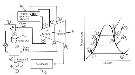
Figure 12.4 A Rankine cycle incorporating reheat and regeneration feedwater heating; both open and closed feedwater heaters are shown (FWH, feedwater heater; HP, high pressure; LP, low pressure).
Regeneration. Regeneration is the process of using the expanding or expanded vapor to preheat liquid before it enters the vapor generator. Although there is no net heat gain to the cycle in doing this, the efficiency of the cycle is increased because the external heat transfer to the working fluid now occurs at a higher average temperature.
Regeneration is accomplished in two ways for Rankine cycles. In the first, some of the vapor that has partially expanded through the turbine is extracted and used to preheat the compressed liquid before it enters the vapor generator. This is called feedwater heating. In the second, the entire flow of vapor leaving the turbine is passed through a heat exchanger (called a regenerator or recuperator) where heat is transferred to the compressed liquid prior to entering the vapor generator. This second type of regeneration requires that the temperature of the vapor leaving the turbine be higher than the condenser temperature.
Two types of feedwater heaters are in common use, and both are depicted in the cycle shown in Figure 12.4. The open feedwater heater preheats the compressed liquid from state 2 to state 3 by mixing in vapor extracted from the turbine at point b. The extracted vapor must be at the same pressure as the outlet of pump l. A second pump is always required on the outflow side to increase the pressure of the compressed liquid to the vaporizer pressure.
A closed feedwater heater preheats the compressed liquid from state 4 to state 5 by heat exchange across a surface. This heater uses vapor extracted from a port in the turbine that is at state a. The pressure of the extracted vapor does not need to be the same as the compressed liquid it is heating. Once condensed, the extracted liquid (called “drips”) is fed back into the main compressed liquid stream, either at a lower pressure open feedwater heater (as is shown in Figure 12.4) or at the condenser.
A full-flow regenerator is included in a Rankine cycle when the temperature of the vapor leaving the expansion device is higher- than the condensing temperature. This is the case for a class of working fluids used in solar Rankine cycles and other low-temperature applications called drying fluids which are discussed in Section 12.2.3. This class of fluids has the characteristic that the entropy of saturated vapor decreases with decreasing pressure, the opposite of steam. Figure 12.5 shows a cycle using full-flow regeneration with a drying fluid.

Figure 12.5 A Rankine cycle using a drying-type working fluid and incorporating full flow regeneration.
When the high pressure saturated vapor of a drying fluid is expanded in an adiabatic reversible process, the temperature of the vapor when it reaches condenser pressure is above the condenser temperature. Because of this temperature difference, the regenerator can exchange heat from the exhaust vapor (state 5 to state 6) to the compressed liquid, raising its temperature from state 2 to state 3.
12.2.2 Components
Vapor Generators. As discussed previously, the designer must choose whether to generate vapor in the receiver of the solar collector or to use an intermediate heat-transfer fluid between the receiver and the vapor generator.
The choice generally depends on the specific design, but there are several primary considerations.
Receiver vapor generators. Generating vapor in the receiver of the solar collector has the advantage of having fewer components and no loss of temperature required with an intermediate transfer. With both liquid and vapor in a receiver, however, extreme care must be taken in the design of the receiver to ensure that the radiant flux incident on that portion of the receiver containing vapor is less than the flux incident in the regions with liquid and where boiling is taking place. This is because the heat-transfer coefficient into a liquid is significantly higher than into superheated vapor. For similar values of solar flux, burnout of the receiver walls could occur in the regions where vapor exists on the other side of the receiver wall.
Many concentrating collector designs require that the receiver change attitude while the collector tracks the sun. This change of attitude increases the chances of high flux on portions of the receiver containing vapor.
Two examples of solar Rankine power systems where the engine
working fluid vapor is generated directly in the receiver are the Solar One
Pilot Plant at
Heat-exchange vapor generators. Use of an intermediate heat-transfer fluid between the receiver and the engine adds complexity and another fluid to the system. Typically, this requires that three separate heat exchangers be used; a preheater, an evaporator, and a superheater. This type of vapor generator is shown in Figure 12.6. Although the mass flow rate of engine working fluid is the same for all three exchangers, the heat-transfer rates are different, not only because of the different heat-transfer coefficients for liquid, boiling, and vapor heat transfer, but also because of the varying temperature differences between the heat-transfer fluid and the working fluid as depicted in the temperature entropy diagram in Figure 12.6.
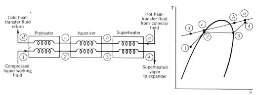
Figure 12.6 Vapor generator (boiler) for a Rankine cycle when an intermediate heat-transfer fluid is used.
Process a-b-c-d depicts the temperature change of the heat-transfer fluid (typically an oil) as it transfers heat in counterflow heat exchangers to the cycle working fluid going from states l-2-3-4. If the superheater is sized properly, the temperature at a will be very close to temperature at 4 (the maximum cycle temperature).
A positive temperature difference everywhere along line ab
c-d
line is required for heat exchange to take place. Therefore, the heat-transfer fluid return
temperature at d cannot be as low as the cycle temperature because of the
requirement that temperature c be above the temperature at 2. The condition at state c is called the pinch
point.
A simplified heat balance of the preheater, the vaporizer and the superheater, respectively gives:
(W) (12.6)
where and
are the mass flow rates of engine working
fluid and heat-transfer fluid, respectively, h represents
enthalpies; T represents temperatures; and cp is the heat-transfer fluid specific heat. The overall rate of heat transfer for each
heat exchanger is represented by
and
. The
total rate of energy transferred to the working fluid is the sum of these three
terms.
Condensers. All power cycles must reject a large percentage of the heat added in order to produce mechanical work. For a Rankine cycle, this heat rejection occurs in conjunction with condensation of the working fluid vapor leaving the turbine at low pressure. The lower the heat rejection temperature, the greater the cycle efficiency as indicated in Equation (12.1).
Heat rejection from the condenser to the surroundings can be either direct or through an intermediate heat-transfer fluid loop (usually water). The types of condensers commonly used in solar power systems are shown in Figure 12.7. The most common condenser, a tube-and-shell heat exchanger, requires a supply of cooling water that comes from either a natural source (river, well, or ocean) or water that has been cooled by a cooling tower. The three cooling towers pictured could be designed either to condense the engine working fluid directly or to reject heat from an intermediate cooling water loop that also circulates through a tube-and-shell condenser.
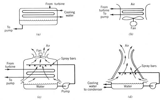
Figure 12.7 Types of condenser and/or heat rejection used in Rankine cycle solar power systems: (a) tube-and-shell condenser; (b) dry cooling tower; (c) wet cooling tower; (d) natural-draft cooling tower.
Each of these heat rejection schemes requires electrical power for operation. This power, considered a parasitic loss from the cycle's output, must be kept to a minimum. Highest parasitic power requirements are usually associated with dry cooling towers since they make use only of the sensible temperature of the air for cooling. This type of cooling is often selected for solar power systems because these systems are often located in hot, arid regions with minimal water resources.
Water evaporation may be utilized to provide additional cooling for the cycle as in examples c and d in Figure 12.7. These units typically provide lower-temperature cooling for less parasitic power than do dry cooling towers. The amount of water resource required may be roughly estimated by assuming that most of the heat rejected by the cycle provides latent heat for evaporation. The rate of water usage by a wet cooling tower may be estimated by
(12.7)
where is the
rate of heat rejection by the cycle and hfg
the enthalpy of vaporization for water (2450 kJ/kg or 1054 Btu/1b).
Expanders. Expanders used most commonly for solar Rankine cycle applications arc turbines and reciprocating piston-cylinder devices. Scroll or screw expanders, rotary-displacement machines (Roots type), and fluid drag disc turbines have also been proposed for small output applications.
The efficiency of an expander is measured relative to an ideal adiabatic, reversible expander. The expansion process of an ideal expander occurs at constant entropy (isentropic). For a real expander, with friction, leakage, and other losses, the entropy of the vapor leaving will be greater than the entropy of the vapor entering. This produces a smaller enthalpy change than would have occurred if the entropy were constant. The isentropic efficiency of an expander, as depicted in Figure 12.8, is written as
(12.8)
where h2 is the actual enthalpy of the vapor leaving the expander and h2s, is the exit enthalpy if the expansion process were isentropic (constant entropy) to the same low pressure. The power output of a real expander is
(12.9)
where is the mass flow rate of vapor through the
turbine.

Figure 12.8 Isentropic efficiency definition for an expander (turbine) and compressor (pump): (a) expander; (b) pump or compressor.
Turbine expanders are most commonly used in solar Rankine cycle systems. Two types of turbine are in common use; the radial-flow turbine and the axial-flow turbine. In radial-flow turbines, the vapor expands from the shaft centerline to the outside periphery of a turbine disc or from outside in. This type of turbine is usually more efficient for small-power-output applications. In axial flow turbines, the vapor flows along the axis of the rotating shaft and passes through blades attached around the periphery of a disc. For large-power-output applications, many axial-flow turbine rotors are stacked together to form a multistage turbine.
Positive-displacement, reciprocating expanders have been proposed for solar power applications. This is the type of expander used in most Rankine cycles a century ago consists of one or more cylinders with pistons driving a rotating crankshaft. In reheat designs, exhaust vapor from a small high-pressure piston and cylinder is reheated in the vapor generator and fed back to a low-pressure piston and cylinder where more expansion work is done.
Pumps. The pump in a Rankine cycle is needed to raise the pressure of the liquid leaving the condenser to the pressure of the vapor generator. A major advantage of the Rankine cycle is that the working fluid is in the liquid phase when it is compressed. Since pump work is inversely proportional to the fluid density, less work is required to pressurize a liquid than a vapor or gas. Since liquids are essentially incompressible, the ideal pump power may be calculated as
(12.10)
where is the mass flow rate through the pump, v
is the fluid specific volume,
p
is the pressure, and h is the enthalpy.
State 2s represents the outlet conditions of an ideal pump, that is, a
constant entropy process. Note that this
expression will give a negative quantity consistent with the sign convention
that work into the cycle is negative.
The ideal pump raises the pressure of a liquid in an adiabatic, reversible process. Real pumps, like turbines, produce an entropy increase in the fluid. Figure 12.8b shows the difference between ideal and real pump performance. As discussed earlier for expanders, the power required to operate a real pump is
(12.11)
Feedwater Heaters. Feedwater heaters use partially expanded hot vapor, extracted from the expander to preheat the working fluid before it enters the boiler thereby increasing overall cycle efficiency. Two types of feedwater heaters are in common use, the open type and the closed type.
An open feedwater heater is simply an insulated mixing chamber where extracted hot vapor is mixed with a flow of compressed liquid. As the vapor condenses, its heat of vaporization is added to the liquid. The chamber must be large enough for this condensation to take place before the liquid reenters the system piping.
A closed feedwater heater is a tube-in-shell heat exchanger in which vapor extracted from the turbine passes on the shell side and condenses, releasing its heat of vaporization to the compressed liquid stream. The condensate is then returned to the compressed liquid stream at a point in the cycle where the pressure is lower.

Figure 12.9 Definition of regenerator effectiveness.
Regenerators. As was shown in Figure 12.5, when a drying fluid is chosen as the working fluid, the vapor leaving the expander still contains heat that can be transferred to the compressed liquid stream since the turbine exit temperature is above the condenser temperature. A vapor-to-liquid heat exchanger, called a regenerator, is typically used for this purpose. The effectiveness of the regenerator is a measure of how well the available temperature difference is utilized. Effectiveness is defined as the ratio of the actual temperature change of the liquid stream to the maximum possible temperature change. Figure 12.9 shows a regenerator and the thermodynamic states of both streams as they flow through the regenerator. The regenerator effectiveness in this case is defined as
(12.12)
where the temperatures are defined on Figure 12.9.
12.2.3 Working Fluid Selection
There are two important aspects to be considered in selecting a working fluid for a Rankine cycle solar power system: (1) to select a working fluid that optimizes cycle efficiency and (2) to match the working fluid states with those of the intermediate heat-transfer fluid if one is used. The effects of different working fluids on these aspects of cycle design are discussed in the following paragraphs.
The Ideal Working Fluid. An ideal working fluid would have the temperature entropy diagram given in Figure 12.10. The following characteristics listed by Abbin and Leuenberger (1974) describe this fluid:
- The
heat capacity of the liquid phase should be small. This makes line 22' in Figure 12.10 almost vertical.
- The critical point should be above the highest operating temperature to allow all heat to be added at that temperature.
- The vapor pressure at the highest operating temperature should be moderate for safety reasons and to reduce the cost of the equipment.
- The vapor pressure at the condensing temperature should be above atmospheric pressure to prevent air leakage into the system.
- The specific volume of the vapor at state 4 should be small to avoid large-diameter turbine wheels, casings, and heat exchangers.
- The saturated vapor line (follows 3-4 in Figure 12.10) should be vertical to avoid expansion into the wet vapor region (negative ds/dT) or expansion into the superheat region (positive ds/dT).
- For low-power turbine applications, the fluid should have a high molecular weight to minimize the rotational speed and/or the number of turbine stages and to allow for reasonable mass flow rates and turbine nozzle areas.
- The fluid should be liquid at atmospheric pressure and temperature for ease of handling and containment.
- The freezing point should be lower than the lowest ambient operating temperature.
- The fluid should have good heat-transfer properties, be inexpensive, thermally stable at the highest operating temperature, nonflammable, noncorrosive, nontoxic, and so on.
Steam. Because it is the most popular Rankine cycle working fluid, more is known about designing Rankine cycle components for steam systems than any other liquid. Because it has a critical temperature and pressure of 374ºC / 22.1 MPa (704ºF / 3206 psia), it can be used for systems operating at fairly high temperatures with most of the heat addition (at constant temperature) and at moderate pressure. The low-temperature characteristics of steam are not quite as ideal since at ambient temperature, steam has a low vapor pressure (0.03 atm) and a very low density. Because of this, it is a major design problem to seal air out of the low-pressure components.
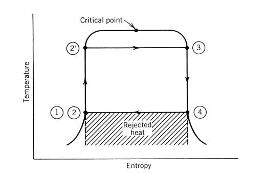
Figure 12.10 An ideal working fluid used with a Rankine cycle.
Steam is a ´wetting fluid´, implying that superheating is required when a turbine is used as the expansion device. As discussed earlier, superheating produces a lower efficiency since most of the heat supplied occurs at a temperature lower than the maximum cycle temperature thereby reducing the average heat-addition temperature.
The major disadvantage of using steam for small Rankine cycles (<1000 kW output) is its low molecular weight (i.e. 18). As is discussed later, in order to attain high turbine efficiencies with low-molecular-weight fluids, very high turbine speeds are called for with small inlet nozzle and blade dimensions.
Because steam is inexpensive to use (although boiler-grade water must be highly distilled and thus costs more than tap water), sealing of the high-pressure portions of a Rankine cycle using steam is not critical. Non-flammability and ready availability of steam are additional advantages. However, its freezing temperature is within the range of ambient conditions. Furthermore, water expands when it freezes, producing large stresses on any structure containing it. Because solar energy systems are located outdoors and are not operational at night, freeze protection or drainage capabilities must be provided for all components in the cycle.
Wetting Versus
Drying Fluids. For some fluids,
the entropy of the saturated vapor increases with increasing temperature. These fluids are called “drying” fluids
because moisture does not form when high-pressure saturated vapor is expanded
reversibly from a high pressure (i.e., in an ideal turbine or nozzle). A notable example used in many solar power
applications is toluene (CH3C6H5). A fluid where
the entropy of the saturated vapor decreases with increasing temperature is
called a “wetting” fluid because moisture forms when high pressure saturated
vapor is expanded reversibly in a turbine or nozzle. The watersteam
combination is a primary example of a wetting fluid. The characteristics of a wetting and a drying
fluid are shown in Figure 12.11, along with real and ideal expansion processes
from saturated vapor.
An ideal fluid, as pointed out in item 6 in the list in the
preceding subsection, would be neither wetting nor drying. Tabor (1962) did an extensive search for
high-molecular-weight fluids that would have an almost vertical saturated vapor
line on temperature-entropy coordinates (ds/dT = 0). A theoretical study showed that the slope of
the entropy-temperature curve was a function of the number of atoms in a
molecule. Molecules with 510
atoms show this tendency. Carbon
tetrachloride, tetrachloroethylene, and monochlorobenzene are all found to have
very small ds/dT
slopes.
As discussed earlier, drying fluids can produce cycle efficiencies almost as great as fluids where ds/dT = 0 if regeneration is used. This is because the higher-temperature heat remaining in the vapor once it has expanded to the pressure of the condenser is not necessarily lost but may be used to preheat the compressed liquid before it enters the vaporizer.

Figure 12.11 Saturation curves for wetting- and drying-type fluid showing ideal and real expansion processes: (a) wetting fluid; (b) drying fluid.
Wetting fluids, on the other hand, will always give less efficient cycles for a given maximum operating temperature because it is necessary to superheat the vapor before it enters the turbine. Superheat is required to ensure that liquid does not form in the vapor as it expands through the turbine. If moisture droplets form, they slow down as they pass through the turbine, finally being hit with great force by the blades. This impact causes erosion of the turbine blades or impeller. Superheat also decreases cycle efficiency because of the lower average heat-addition temperature.
Molecular Weight. The desire for using a heavier molecular weight fluid for small power cycles (item 7 in preceding list) derives from basic turbine design considerations. The most important are the turbine speed, the number of stages, and the size of the flow passages. Proper selection of these is required to design an efficient turbine. A detailed development of turbine design parameters may be found in Baljé (1962).
The data in Table 12.1 show that for turbine power levels of less than 1 to 10 MW, the isentropic efficiency of a steam turbine is considerably lower than that of a turbine designed for heavy-molecular-weight fluids. The reasons why high turbine efficiency cannot be maintained for low-power-level designs using a low-molecular-weight fluid are
1. The first stage nozzle spouting velocity is inversely proportional to the square root of the molecular weight. Since the ratio of blade speed to fluid speed must remain relatively constant, multiple staging and high rotational speeds are called for when low-molecular-weight vapors are used. The added complexity and expense of multi-staging is inappropriate for small turbines because disc friction, leakage, and windage losses become prohibitive in small designs.
2. The volumetric flows in the initial stages of the turbine are proportional to the square root of the molecular weight and therefore low with low-molecular-weight vapors. This requires the use of small nozzles, blades, and flow passages. Partial admission may be used, but this reduces efficiency. Also, blade tip, sealing, and boundary-layer losses become significant in small designs. Even with the use of precision manufacturing techniques, small turbine stages result in a turbine with low efficiency.
Table 12.1. Comparison of Turbine Isentropic
Efficiencies Using Steam (Low Molecular Weight) and
a High Molecular Weight Working Fluid
|
Power Level |
Turbine lsentropic Efficiency (%) |
|
|
|
Steam |
High Molecular Weight |
|
>10MW |
70-80 |
75 |
|
1-5 MW |
50-70 |
75 |
|
200-500 kW |
30-50 |
75-80 |
|
10-100 kW |
25-50 |
60-75 |
Source. Abbin (l983).
Fluid Properties. A primary consideration in selecting a Rankine cycle working fluid is the saturation pressure at the high and low operating temperature. At both of these temperatures, the pressure must be less than the critical pressure and not extremely high or low as discussed in items 3 and 4 in the preceding list for the ideal fluid. For solar applications, the maximum operating temperature varies widely depending on the type of solar collector being used. Table 12.2 presents data on some working fluids that have been used or considered for use in Rankine cycles.
Table 12.2. Physical and Thermodynamic Properties of Prime Candidate Rankine Cycle Working Fluids
|
|
|
|
2-Methyl |
Fluorinol |
Toluene |
Freon |
Freon |
|
Molecular weight |
18 |
32 |
33 |
88 |
92 |
137 |
187 |
|
Atoms per molecule |
3 |
6 |
14 |
9 |
15 |
5 |
8 |
|
Boiling point (1 atm) (ºC) |
100 |
64 |
93 |
75 |
110 |
24 |
48 |
|
Liquid density (kg/m3) |
999.5 |
749.6 |
934 |
1370 |
856.9 |
1476 |
1565 |
|
Specific volume (saturated vapor at boiling point) (m3/kg) |
1.69 |
0.80 |
0.87 |
0.31 |
0.34 |
0.17 |
0.14 |
|
Maximum stability temperature (ºC) |
--- |
175-230 |
370-400 |
290-330 |
400-425 |
150-175 |
175-230 |
|
Wetting-drying |
W |
W |
W |
W |
D |
Both |
D |
|
Heat of vaporization |
2256 |
1098 |
879 |
442 |
365 |
181 |
146 |
|
Isentropic enthalpy drop across turbine (kJ/kg) |
348-1160 |
162-302 |
186-354 |
70-186 |
116-232 |
23-46 |
23-46 |
Source. Marciniak et al. (1981).
The relationship between saturation pressure and the saturation temperature can be approximated as
(12.13)
The boiling pressure at any temperature can be found by applying Equation (12.13) from the critical conditions and one other data point. Figure 12.12 shows the saturation lines for a wide range of potential Rankine cycle working fluids.

Figure 12.12 Saturation pressure-temperature relationships for potential Rankine cycle working fluids.
For extremely high temperature applications, liquid metals have been used as Rankine cycle working fluids. A liquid metal "topping" cycle would reject heat to a second, lower-temperature “bottoming” cycle. As can be seen in Figure 12.12, the saturation temperature of this class of working fluids is very high. However, they are of interest to the solar designer both as a Rankine cycle working fluid and as a high-temperature intermediate heat-transfer fluid.
Tabulated thermodynamic property data for a large number of potential working fluids are available to the designer, in Reynolds (1979) or from the companies that manufacture the fluids. Because of their importance as a small power system working fluid, thermodynamic property data for steam and toluene (CH3C6H5) are included in the Appendix.
Thermodynamic properties may also be calculated. Computer calculation of properties is often useful when a great number of cycles or fluids are to be analyzed. A description of these computational procedures is beyond the scope of this book. The interested reader is referred to Abbin and Leuenberger (1974) for a relatively simple approach to analytical property prediction and to Reynolds (1979) for more extensive algorithms.
12.2.4 Cycle Thermal Design
Cycle thermal design involves construction of a cycle diagram on thermodynamic coordinates by locating the thermodynamic states of the working fluid as it enters and leaves each component. In order to define these thermodynamic states, the designer has few choices once the maximum and minimum cycle temperatures have been defined and the working fluid chosen.
Average Heat-Addition Temperature. One choice remaining is to maximize the "average" heat-addition temperature. This pseudo-temperature helps the designer visualize the combination of cycle heat-addition processes (preheat, boiling, and superheat) that maximize cycle efficiency. The average heat-addition temperature is defined as the temperature that produces the same area as the area under a heat addition process curve on T-s coordinates. In analytical terms, this temperature is represented by the following:
(12.14)
where states 1 and 2 represent the initial and final states of the heat transfer process.
The Pinch Point. When an intermediate heat-transfer fluid is used, heat addition to the working fluid takes place in three counterflow heat exchangers as shown in Figure 12.6. The processes are again depicted on Figure 12.13 with the scale distorted for clarity. The heat-transfer fluid at a represents the solar field outlet temperature and at d, the field return temperature. The difference between these can be reduced by increasing the flow rate of heat-transfer fluid through the field and thus the parasitic pumping power.

Figure 12.13 The working fluid vaporization process using an intermediate heat transfer fluid in countertlow heat exchangers.
The slope of curve a-b-c-d (and the parasitic pump power) is defined by states 2 and 4 of the cycle working fluid. Since a heat exchanger must always have a positive temperature difference to transfer heat, the temperature of the intermediate heat-transfer fluid must always be above the temperature of the working fluid. Point a represents the maximum solar collector field temperature and point 4 the maximum cycle temperature. Points c and 2, called the pinch point, define the lowest temperature (point d) at which heat transfer fluid can be returned to the collector field.
It is important to make the difference (TaTd) large to
reduce the heat-transfer fluid flow rate and hence the parasitic pumping power
required for the solar collector field.
This can be done by increasing the amount of superheat given to the
cycle working fluid. Increase in the
amount of superheat for the cycle reduces the solar field pumping power. However, increase in superheat for a given
maximum cycle temperature reduces the power cycle efficiency but increases the
solar collector efficiency by reducing the average heat-addition temperature as
defined in Equation (12.14). The result
is that the cycle designer is faced with a tradeoff between cycle efficiency
and collector field efficiency and must find an optimum solution.
Cycle Design Procedure. The cycle design procedure differs for wetting and drying working fluid. The procedure can best be explained on the temperature- entropy (T-s) coordinates in Figure 12.14. For simplicity, the finite heat-exchange temperature differences required at c and d are not shown.

Figure 12.14 Cycle design sequence: (a) for a wetting-type fluid; (b) for a drying-type fluid.
Wetting fluids. For a wetting fluid when an intermediate heat-transfer fluid is used, the cycle design procedure follows this sequence (the letters refer to states noted in Figure 12.14a):
a - Once the working fluid has been selected and the maximum and minimum cycle temperatures have been defined, the most important cycle design criterion is the amount of moisture permitted at the exit of the expander (turbine). High moisture content (low quality) at this point causes erosion of the blades or impeller and inefficient operation. This point is shown in Figure 12.14a as state a.
b, c - The isentropic turbine exit state b, is then calculated as
(12.15)
where the turbine efficiency ηt must be known and state c will be at the intersection of the maximum cycle temperature and a vertical line from b. This is an iterative procedure but converges rapidly. In some design situations such as total energy systems where the condensing temperature is purposely high, the pressure at i may be too high for reasonable component design. This forces the cycle designer to a new, less efficient turbine inlet condition c’ and redefines points b and a.
d - With the definition of point c,
the pressure at which heat addition takes place is defined. Since most of this heat transfer takes place
at the boiling temperature d, the average heat-addition
temperature TH is now fixed.
If the lower turbine inlet pressure at c' (with more
superheating) had been selected,
TH would have been lower,
resulting in a less efficient cycle.
e, f - The pump exit condition is now defined by the vaporizer pressure and a vertical line from the saturated liquid point at the condensing temperature (point f). Actually this is not a vertical line for real pumps, but it makes little difference in the cycle design.
g - Finally, the heat-transfer fluid temperature line is drawn above points c and d. Its slope and thus the fluid return temperature at g are defined by the maximum collector temperature and the pinch point temperature.
It should be noted here that the assumption that line d-g is a continuation of line c-d is not exact due to differences in heat transfer for the two processes.
Precisely, the temperature of the heat-transfer fluid leaving the heat exchanger will be slightly higher than g but less than d. Its true value may be determined by an enthalpy balance of the preheater section of the heat exchanger; however, this is not necessary in cycle design.
If the difference between the field output temperature and the return temperature is so small that high field flow rates are required, the cycle pressure must be reduced to c', and the resulting field return temperature at g' will be lower. This will also make the cycle efficiency lower.
Drying fluids. When the cycle working fluid is a drying fluid and an intermediate heat-transfer fluid is used, the cycle design procedure reverses. Ideally, to obtain the highest cycle efficiency, no superheat would be used and TH would be very close to the maximum cycle temperature. However, now the parasitic solar field pumping loss and hence the minimum field temperature rise becomes the determining factor for the entire cycle design once the maximum and minimum temperatures have been set. The process is as follows (see also Figure 12.14b):
On a vertical line from the condensed liquid state, define point a representing the highest collector field return temperature permitted without requiring excessive pumping power in the collector field loop.
A straight line is drawn from point a that just touches one of the constant pressure lines at b and again at c, where it also intersects the maximum temperature line simultaneously. There is only one saturation pressure curve that will meet these criteria, and this will be the cycle high pressure. At excessive pressures, the pinch point condition will be violated and at insufficient pressure the cycle efficiency will be reduced since the average temperature of heat addition will be lower.
A vertical line is now dropped from point c to point d, its intersection with the condensing pressure. This line represents the isentropic turbine expansion.
Point e, the actual turbine exit condition is defined at the same pressure by the turbine exit enthalpy from
(12.16)
and the cycle is completely defined. The actual collector field return temperature will be slightly higher than a and iterative techniques must be used for the final cycle design.
A Comparative Cycle
Design Table 12.3. Comparison of Toluene and Steam Solar Power Steam Toluene Thermodynamic cycle: High temperature 340ºC 340ºC Power output 100 kW 100 kW Ideal efficiencya 40.8% 34.8% Turbine: Stages 2 4 Speed 25,000 rpm 50,000 rpm Medium blade
diameter 19.1 cm 11.3 cm First-stage nozzle
area 7.7 cm2 0.58 cm2 Isentropic
efficiency 72.5% 68.0% Power cycle efficiency:b 24.2% 20.1 % Overall plant efficiency:c 15.1% 12.5% SOURCE: Schmidt et al. (1983). aIdeal Rankine cycle. bIncludes engine component efficiencies. cIncludes 73 percent efficient collectors, field heat
loss, and tracking and control parasitics. An example of one such comparison between steam and toluene
was performed for the design of a point focus, central plant solar power system
now operating in It can be seen in Table 12.3 that there are advantages in
the use of toluene, both in the thermodynamic cycle design and in the design of
the turbine. Note that the resulting
turbine for the toluene cycle was larger in diameter, lower in speed, and less
complex (fewer stages). This results in higher
turbine efficiency (and probably a lower cost). After applying all the parasitic energy losses, the final
toluene cycle efficiency is higher, giving a higher overall system efficiency
(which includes collector and field piping losses). In selecting the toluene
design, the advantages and disadvantages of each fluid are summarized below: 1.
Advantages - toluene: ·
Small turbine head allows for moderate shaft
speed and a single- or two-stage design. ·
Low volume ratio facilitates the flow path
design. ·
High volume flow and low velocity of sound
results in reasonable flow areas. ·
Low temperature drop during expansion reduces
thermal stress problems. ·
Dry expansion avoids blade erosion caused by
vapor wetness. ·
Low system pressure facilitates housing design. 2.
Advantages ·
Well-established design procedures available. ·
Well-known fluid properties. ·
Sealing of shaft housing not critical. 3.
Problem areas ·
Limitation of turbine head due to low velocity
of sound (Mach number of rotor blades). ·
Adequate sealing and ventilation required
because of flammability and toxicity of fluid. 4,
Problem areas ·
Very small nozzle dimensions call for partial
admission and very high shaft speed. ·
High turbine head calls for multistage turbine. ·
High volume ratio imposes problems on the flow
path design. ·
High-performance turbines not available. In a major study of Rankine cycles using different fluids,
Marciniak et al. (1981) concluded that for temperatures below 371ºC (700ºF),
steam Rankine cycles become less efficient and more expensive than organic
fluid cycles. No significant health or
safety problems were foreseen for the working fluids studied (methanol,
2-methylpyridine/ H2O, Fluorinol 85, Toluene, and Freon R-11 and R-I l3). The
major disadvantages of these fluids is their relatively low thermal stability
temperature and potential material compatibility problems. The advantage of using organic working fluids in Rankine
cycles of small sizes and operating at low temperature can be summed up in
terms of the following properties (Abbin, 1983): (1) high molecular weight
results in simpler, more efficient low-power turbine expanders; (2) low
freezing point and no expansion on freezing; (3) high vapor pressure at low
temperature reduces air leakage contamination; and (4) heat-addition
characteristics can be closely matched to the heat-source characteristics. Cycle analysis is the process of determining the properties
of the working fluid as it passes through the various processes in the
cycle. Once the properties at each state
have been determined, the size of the components may be determined along with
the rate of heat transfer or work to or from each. The overall thermodynamic cycle efficiency
may then be calculated. The sequence required for this analysis is presented as an
algorithm that could readily be incorporated into a cycle analysis computer
program. However, a method of inputting
working fluid thermodynamic properties at the various states must also be
incorporated. Some thermodynamic property algorithms were discussed in
Section l2.2.4. Because these algorithms are complex or require significant
storage and processing time, a full cycle analysis computer program is not
included here. The interested designer
could develop such a program by combining the cycle analysis algorithm given
here with a thermodynamic properties algorithm considered appropriate for the
application. Many companies have
developed such programs, and at least one code, has been reported by Abbin and
Leuenberger (1974). Cycle analysis usually starts with knowing the net output
power required from the cycle along with the vapor generator (boiler) exit and
condenser exit states. These are
determined by the cycle design procedures discussed in the previous
section. Turbine and pump isentropic
efficiencies are either known or assumed. The next steps involve determination of the thermodynamic
state (and properties) of the working fluid at the inlet and outlet of each
component in the cycle. The most
important property to be found is the enthalpy. At this point the cycle thermodynamic efficiency may be
determined since it does not depend on the size of the components. Component sizing is then done by calculating
the mass flow rate required for the defined output power. Finally, the rate of energy transfer for each
component may be calculated. Since this procedure differs for each cycle configuration,
each configuration is treated separately in the following subsections. No
parasitic pressure drop or heat loss is included but could be added if
considered significant. The Simple Rankine
Cycle. The simple Rankine cycle
has only four components, a pump, a vaporizer, an expander, and a condenser as
shown in Figure 12.15. The working fluid is a wetting working fluid (the drying
fluid usually incorporates regeneration and is discussed later). The vapor
leaving the vaporizer is shown to he superheated. If the vapor is not
superheated, the saturated vapor quality at the turbine exit must be specified
and becomes the second property for specification of state 3. A complete cycle
analysis algorithm for this cycle is given in the Appendix. Figure 12.15 A simple Rankine cycle with superheated vapor
at the turbine inlet. Rankine Cycle with
Reheat. Reheat is often included
in large Rankine cycles using wetting fluids so that the boiler can operate at
higher temperatures and still provide for low moisture content at the turbine
exit. To accomplish this, two turbines
are used, often on the same shaft. A
cycle diagram depicting this is shown in Figure 12.16. Vapor exits from the first expander; returns
to the vaporizer, where it is reheated to its original temperature (but at a
lower pressure); and enters a second expander, where the pressure drops to the
condenser pressure. The complete cycle
analysis algorithm for this cycle is given in the Appendix. Figure 12.16 A Rankine cycle with reheat of the partially
expanded vapor. Rankine Cycle with
Open Feedwater Heating. With
open feedwater heating, a small percentage of partially expanded vapor is
extracted from the turbine and mixed directly with the compressed liquid
(feedwater) to preheat it before going into the vaporizer. A Rankine cycle incorporating an open feedwater
heater is shown in Figure 12.17. The
extraction flow at 6 is determined by the amount of heat required to raise the
temperature of the feedwater from state 2 to state 3. Because the mass flows
are different at different points in the cycle, analysis of the cycle becomes
slightly more involved. The complete
cycle analysis algorithm for this cycle is given in the Appendix. Figure 12.17 A Rankine cycle with open feedwater heating of
the compressed liquid. Rankine Cycle with
Closed Feedwater Heating. A Rankine cycle with a closed feedwater
heater is shown in Figure 12.18. Again the rate of extraction flow at 5 is
determined by the enthalpy rise required between states 2 and 3. The condensation from the feedwater heater
(called “drips”) in this example is
throttled through a liquid trap back in the condenser at 8. An alternative used sometimes would be to
replace the trap with a small pump and reinject the condensate at state 2. A complete cycle analysis algorithm for this
cycle is given in the Appendix. Figure 12.18 A
Rankine cycle with closed feedwater heating of the compressed liquid. Rankine Cycle with
Regeneration. When a drying fluid is used as the working fluid, the
turbine exit stream is at a higher temperature than the pump exit
temperature. Instead of being placed
directly in the condenser, the turbine exhaust can first pass through a heat
exchanger with the waste heat being used to preheat the compressed liquid
before it enters the vaporizer. This
heat exchanger, called a regenerator or a recuperator, is shown in Figure 12.19. The cycle analysis algorithm for this cycle
is given in the Appendix. Figure 12.19 A Rankine cycle with full-flow regeneration
using a drying-type working fluid. Most solar power cycles in operation or under development
today are Rankine cycles. We discuss the
important cycle design characteristics of four of these below. Each represents an optimum solution to a
different design problem in terms of maximum temperature, power output, or
external demands. Their characteristics
are summarized in Table 12.4. Table 12.4. Characteristics of Selected Solar Rankine Power Cycles Parameter Coolidge Shenandoah Dish ORC Solar One Tmax 268ºC 382ºC 400ºC 516ºC Tcond 40.5ºC 110ºC 45ºC 43ºC Power 240 kW 430 kWa 26 kW 12,900 kW Working fluid Toluene Steam Toluene Steam Heat-addition method Heat transfer fluid Heat transfer fluid Receiver boiling Receiver boiling Cycle efficiency 24% 17%b 24% 35% Percent of Carnot 57% 41% 45% 58% Turbine inlet state 50ºC of superheat 117ºC of superheat 103ºC of superheat 198ºC of superheat Regeneration Regenerator 1 FWHc Regenerator 4 FWHc Turbine stages 1 4 1 17 Mean turbine diameter 58.7 cm 10.2 cm 12.5 cm 64.5 Speed 9300 rpm 42,480 rpm 60,000 rpm 3600 rpm aPlus bleed process steam and absorption chiller heat. bNot including bleed or chilling. cFeedwater heaters (FWH). Coolidge Irrigation
System. The cycle designed for the Coolidge ( The maximum efficiency of this cycle is 24 percent, which is
57 percent of the efficiency of a Carnot engine operating at the same peak
temperatures. The power cycle was built by
Sundstrand, Inc. and is a modified version of a commercial power cycle used for
waste heat recovery. This solar energy
system is described further in Chapter 16. Shenandoah Total
Energy System. The power cycle
at the Shenandoah (Georgia) Solar Total Energy Project is a Rankine cycle using
superheated steam. Heat is supplied from
a field of parabolic dishes by an intermediate heat-transfer fluid. One open feedwater heater is used in a cycle
that resembles that shown in Figure 12.17. Operating with a maximum turbine
inlet temperature of 382ºC (720ºF), the system is designed to produce 430 kW of
shaft power in addition to providing process steam at 173ºC (343ºF) and a high
heat-rejection temperature to operate an absorption chiller. The requirement for process steam and a high condenser
temperature forced the design toward the use of steam even though the power
output and operating temperature are in the range where organic fluids usually
prove optimum. The steam entering the
turbine has been superheated by 117ºC (211ºF). The turbine developed for this
system by Mechanical Technologies, Inc. consists of a two-stage axial-flow
high-pressure section and a two-stage axial-flow low-pressure section with a
mean blade diameter of l 0.2 cm (4 in.).
At maximum power, the turbine rotates at 42,480 rpm. The overall power cycle efficiency is 17 percent which is 42
percent of the maximum possible. However, this efficiency value does not
include the useful energy in the steam bled for process steam or the high-temperature
rejected heat used to power an absorption cooler. This solar energy system is
described further in Chapter 16. Small Communities
Project. The organic Rankine
cycle designed for the U.S. Department of Energy's Small Communities Project by
Barber-Nichols Engineering is designed to be placed at the focus of a single
parabolic dish concentrator. This small
regenerative unit has a cycle similar to that pictured in Figure 12.19. It is designed to produce 26 kW of shaft
power with a peak operating temperature of 400ºC (752ºF). The working fluid is toluene. However, the operating temperature approaches
the limits of this fluid, and over 100ºC (180ºF) of superheat is used to take
advantage of the temperature capability of the parabolic dish heat source. Figure 12.20 The turbine, alternator, and pump assembly for
the Barber-Nichols solar Rankine cycle engine module. In order to enhance the efficiency of such a small system,
the turbine, pump, and alternator are incorporated on the same shaft as pictured
in Figure 12.20. This concept also
eliminates a dynamic shaft seal, enhancing its service life. The single-stage, axial-flow turbine spins at
60,000 rpm and has a mean blade diameter of 12.5 cm (4.9 in.). This engine has
a thermal efficiency of 24 percent which is 45 percent of the ideal Carnot
efficiency. Solar One Pilot
Plant. The design conditions for the Solar One central receiver pilot
plant, meet the steam Rankine cycle minimum of both power and temperature
discussed in Section 12.2.3. Operating
at a maximum temperature of 516ºC (916ºF) and producing 12.9 MW of shaft power,
the working fluid choice was steam. The steam boils and is superheated in the
receiver, thus eliminating the need for an intermediate heat-transfer fluid and
resulting pinch point matching problems.
Four stages of feedwater heating are used, three closed and one an open
deaerator as depicted in Figure 12.21.
The turbine for Solar One has 17 axial-flow stages with blade diameters
of 32.3 to 57.7 cm (12.7 to 22.7 in.), using blades 2.23 to 15.5 cm (0.89 to 6.11
in.) long. The turbine turns at 3600 rpm, which is the normal speed for most
large-scale steam electric power generating plants. At these conditions, this cycle has an
overall efficiency of 35 percent, which is 58 percent of the ideal cycle
efficiency at these operating conditions.
Additional details of the design of this system are given in Chapter 16.
Figure 12.21 Schematic of the l0-MWe steam Rankine cycle at
the Solar One pilot plant at The The Ideal Cycle.
The ideal Figure 12.22 The four
processes of an ideal In the ideal cycle, heat is rejected and work is done on the
working fluid during the isothermal compression process 1-2. For a fixed mass of working fluid, the amount
of total work required for this process is represented by the area 1 Because more work is done by expanding a gas at high
temperature than is required to compress the same amount of gas at a low
temperature, the The only difference between the The amount of work and heat transfer for each process of an
ideal where p is the pressure, V
is the total volume, TL
is the cycle low temperature, Similarly, for the high-temperature expansion process and where this time the quantity is positive since Equations
(12.19) and (12.20) represent work done by the system and heat added to the
system. The total heat that must be saved and transferred by the
regenerator is where cv, is the specific heat at constant volume of that
particular gas per unit mass. The net work produced by the cycle is and it can be shown by combining Equations (12.22) and (12.20),
that the cycle efficiency reduces to which is exactly the Carnot cycle efficiency. The design of a
mechanical device that performs the cycle depicted in Figure 12.22 is not an
easy task. Because of the constant volume compression and expansion processes
involved, a reciprocating piston-cylinder arrangement is normally used. According to Martini (1980) traditional Figure 12.23 Main types
of The alpha-type
uses two pistons. These pistons mutually compress the working gas in the cold
space; move it through a regenerator to the hot space where it is expanded; and
then move it back to the cold space, completing the cycle. A variation called the Rinia arrangement uses double-acting pistons with the compression
space, which is a sealed chamber on the back side of the adjacent piston. Four such pistons are connected together in
the United Stirling Model 4-95 engine currently being tested for solar power
applications. The beta and gamma types use a power piston and a
displacer piston. The power piston does
the compression and expansion of the gas, and the displacer pushes the gas from
the hot to the cold space and back. The
displacer arrangement with the displacer and power piston in line is called a beta-arrangement. When the power piston is offset from the
displacer to provide a simple mechanical arrangement, it is called a
gamma-type. In the example shown of this
type, the regenerator moves through the gas rather than using a displacer to
move the gas through the regenerator. In practice, the processes occurring in the engines are not
ideal. Figure 12.24 shows a typical pressure Figure 12.24 Cycle diagram showing typical real processes of
a One of the major causes of inefficiency in the where the subscripts H, L, and R refer to the
high, low, and regenerator temperatures, respectively. Here TR
is the mass-averaged gas temperature leaving the regenerator during
heating. The heat transfer from the
regenerator to the gas no longer is expressed as Equation (12.21) but becomes The remainder of the heat required to raise the working gas
to its high temperature is supplied by the external heat source and is The total amount of heat input to the cycle is the sum of
Equations (12.26) and (12.20): The cycle efficiency for a where k is the ratio of specific
heats (cp/cv). Regeneration is not necessarily required for a The other major cause of Calculation of the cycle efficiency and other engine design
parameters for a The choice of a working gas for a In developing the The Solar 4-95 Figure 12.25 The
United Stirling Model 4-95 solar The 4-95 engine has four double-acting pistons in an
alpha-type Rinia arrangement where the top (hot) chamber works in conjunction
with the bottom (cool) chamber of an adjacent piston through the heater,
regenerator, and cooler. The heater
consists of 72 small-diameter tubes shaped in a cone that forms the back side
of a cavity receiver. These tubes
connect the cylinder to the regenerator.
Concentrated solar flux is absorbed directly on the heater tubes, thus
precluding the necessity of intermediate heat-transfer surfaces or fluids. The heater operates at 720ºC (1328ºF). Cooling is provided by a cool water supply. The cool chamber behind the piston is sealed from the
crankcase with the piston rod passing through a linear seal. Linear motion of
the rod is maintained by a crosshead that then connects to the crankshaft,
which rotates at 1800 rpm. Either
hydrogen or helium may be used as a working fluid. Power control is attained by increasing or
decreasing the mean pressure of the working gas in the cycle. Constant heater temperature is maintained
through this control system since the engine speed is fixed by the 60 Hz power
grid. At an output power of 25 kW, the
maximum gas pressure is 18 MPa (2611 psia). Sealing of reciprocating engines to prevent gas leakage has
been a major Figure 12.26 shows an example of a free piston Figure 12.26 A free
piston Brayton cycle engines are being considered for both small-
and large-scale power applications. The major advantage of this type of engine
is the potential for low operation and maintenance costs. This engine has been
proposed for parabolic dish power modules, where a small engine is mounted at
the focus of the concentrator, and for central receiver systems where
pressurized gas is heated in the central
receiver. Operating at relatively low
pressures, the Brayton engine requires large, hot gas receivers. The major drawback to their implementation is
the high receiver operating temperatures required to get reasonable
efficiencies. Most Brayton engines are
not self-sustaining at operating temperatures below 480ºC (900ºF). The ideal simple Brayton cycle shown in Figure 12.27
combines four thermodynamic processes for the working fluid. An adiabatic, reversible (and thus
isentropic) compression process from states 1 to 2 raises the pressure of the
working fluid from the cycle low pressure to the high pressure. Heat is then added at constant pressure (2-3)
until the maximum cycle temperature is reached.
An adiabatic reversible expansion then takes place (3-4) through an
expander (usually a turbine), where work is produced. The low-pressure gas is
then cooled at constant pressure to the inlet conditions of the compressor
(process 4-1). Figure 12.27 The four
processes of an ideal simple Brayton cycle engine. The heat transfer for these processes may be visualized on
the temperature For the ideal simple Brayton cycle, cycle efficiency is
determined only by the pressure ratio across the compressor (or turbine). The cycle efficiency is Figure 12.28 shows the variation of cycle efficiency with
engine pressure ratio for both a diatomic gas such as air and a monatomic gas
such as helium, argon, or neon. Helium
has been proposed for solar Brayton cycles because of its obvious efficiency
advantage plus its high heat transfer capability and because it is inert. Figure 12.28 The
ideal simple Brayton cycle efficiency for monatomic and diatomic gases. Figure 12.29 shows the physical arrangement of the
components of a Brayton cycle engine.
When air is the working fluid, Brayton cycles may be either open or
closed cycles. If closed, process 4-1 is
carried out in a heat exchanger, where heat is transferred from the working gas
to ambient conditions. If the cycle is
open, warm air is dumped from the turbine exhaust into the surroundings at
state 4 and cool ambient air (at state 1) is drawn into the compressor. For large-scale, open Brayton cycle engines,
it is essential for there to be natural air movement past the site to prohibit
reinjection of the warm exhaust. If a
working gas other than air is used, a closed cycle is required. Figure 12.29 Simple
Brayton cycle engines. Both open and
closed cycles are shown. In solar applications, the receiver is the heater and hence
will be pressurized to the cycle high pressure if no intermediate heat-transfer
fluid is used. Since ideal cycle
efficiency is only a function of the pressure ratio and not the actual
pressure, a Brayton cycle with process 2 If the turbine exit temperature (T4 in Figure 12.27) is higher
than the compressor exit temperature T2,
heat may be transferred from the exhaust stream to preheat the compressed gas
before heat addition. This process is
called regeneration or recuperation. The regenerative Brayton
cycle is shown in Figure 12.30. Figure 12.30 A
regenerative Brayton cycle. Regeneration
is possible when T5 is greater than T2.
The maximum pressure ratio for which regeneration is
possible may be defined in terms of the maximum and minimum cycle temperature
as The cycle efficiency for an ideal regenerative Brayton cycle
is not only a function of the cycle pressure ratio, but also the ratio of the
minimum to maximum absolute cycle temperature as given by Figure 12.31 compares the efficiency of an ideal
regenerative cycle with the simple Brayton cycle. It can be seen that for a temperature ratio
of 4 and a working gas with k = 1.4, engines with pressure ratios below 11.31
have a higher efficiency when regeneration is used. In fact, for the limiting case of engines
with a pressure ratio of unity, the regenerative engine will attain the Carnot
cycle efficiency for that temperature (75 percent). The conclusion one reaches from these studies is that the
highest-efficiency Brayton cycles are regenerative cycles with low pressure
ratios. If regeneration is not used,
high pressure ratios are required to provide high efficiency. Finally, for a given temperature ratio, there
is a pressure ratio beyond which regeneration cannot be used since the turbine
exhaust temperature is lower than the compressor outlet temperature. Real engine considerations modify these
conclusions somewhat, as is discussed below. Figure 12.31 The
regenerative Brayton cycle efficiency compared with the simple cycle
efficiency. Regeneration is not possible past the point where the two curves
intersect. In an attempt to develop an engine based on the Brayton
cycle that has an efficiency approaching that of the Carnot cycle, the simple
Brayton cycle may be modified by combining a number of stages of compression in
series with coolers (called intercoolers)
between each stage. Likewise, the
expansion process is staged with the gas being reheated between each
stage. Regeneration between the last
turbine stage and the last compressor outlet is also used. Maximum efficiency is attained when equal
pressure ratios are maintained across each compressor and each turbine stage. An example of multi-staging is shown in Figure 12.32, where
two stages are illustrated. The end
result of multi-staging is that the heat-transfer processes occur at a higher
average temperature. In the limit, with
a large number of stages, the resulting cycle approaches a cycle consisting of
two constant-pressure processes and two constant-temperature processes. This
cycle, called the Ericsson cycle, has
the potential of attaining Carnot efficiency as long as regeneration is used. Figure 12.32 A
multistage Brayton cycle engine with intercooling and regeneration. The efficiency of the multistage Brayton cycle shown in
Figure 12.32 is the same as the efficiency of either of its sections. The heat transfer and work are simply the sum
of' that required for each section. The
major advantage of multistaging is
that the engine can have the high efficiency associated with low-pressure ratio
regenerative cycles (see Figure 12.31) without the extremely large regenerator
required for a single-stage cycle of the same power output. So far we have considered only cycles consisting of ideal
components. In actual Brayton cycle
engines, there are three major losses that have an important effect on the
actual engine efficiency: duct pressure losses, turbomachine efficiencies, and
regenerator effectiveness. Because the working fluid for a Brayton cycle is a gas, very
high volume rates are required for production of desired power levels. This requires large ducts between components
and in the heater and regenerator. With
most designs, there is a significant pressure drop in the heater. When regeneration is used, there is a
pressure drop across the regenerator. These drops are shown in Figure 12.33
where states 2, 3, and 4 as defined in Figure 12.30 are at different pressures. This reduces cycle efficiency by reducing the
pressure drop across the turbine.
Similarly, the turbine exit must be at a higher pressure than the inlet
in order to drive the gas through the regenerator and to cause it to flow away
from the engine. In an open cycle, the
turbine exit pressure p5, is significantly above atmospheric pressure and the
compressor inlet pressure p1, below ambient pressure. In cycle analysis, these pressure losses are combined into a
single factor called the ducting (or
pumping) efficiency. Using the state designations of Figure 12.33, we can
define the ducting efficiency is as As discussed for Rankine cycles, the turbine or compressor
efficiency may be expressed in terms of the actual enthalpy drop across the
machine compared to the enthalpy drop for an isentropic process between the
same two pressures. The efficiency of the compressor shown in Figure 12.33 may
be visualized as the ratio between the lengths of line 1-2s and line 1-2. State 2 will always have higher entropy than
state 1 unless significant quantities of heat are removed during the
compression process. Likewise, the
turbine efficiency is represented by the difference between lines 4 Figure 12.33 Real
engine processes showing the effects of duct pressure loss, compressor and
turbine efficiency, and regenerator effectiveness. If a constant specific heat is assumed, the turbine
efficiency may be written as A similar expression may be written for the isentropic
efficiency of the compressor. The third source of deviation between ideal and actual cycle
processes is the regenerator effectiveness.
Also discussed in detail in the Rankine cycle section above, the real
regenerator will not raise the compressed gas stream to the maximum possible
temperature T5. Instead, the temperature of the pressurized
gas stream leaving the regenerator will be some value, T3, less than T5. For the regenerator shown in Figure 12.33,
the effectiveness of regenerator is To account for these effects in predicting cycle efficiency,
a cycle analysis is normally performed. A cycle analysis algorithm for the Brayton cycle is
presented in the Appendix. As with Rankine cycle analysis, the cycle designer
must choose the method of determining the gas properties according to the level
or accuracy desired. The simplest choice
is a constant specific heat. This is
usually adequate for monatomic gases (helium, argon, and neon). Since specific heats of diatomic gases (i.e.,
air and hydrogen) vary with temperature, a temperature-dependent function
should be used based on data given in the Appendix. Analysis of a simple Brayton cycle starts with definition of
the inlet conditions, the compressor pressure rise, and the maximum cycle
temperature. In addition, the component
efficiencies must be specified along with the net power required from the
cycle. Temperatures and pressures are
then calculated for every point in the cycle.
The cycle is sized by calculating the working gas flow rate required for
the desired power output. The work or
heat flows for each component may then be calculated. Since the cycle analysis procedure is almost the same for
simple, regenerative, and multistage Brayton cycles, only one algorithm is
given in the Appendix. When regeneration
is not used as with the simple cycle, the effectiveness of the regenerator is
set equal to zero. For multistage
cycles, the cycle efficiency is the same as for each compressor-turbine stage
using maximum regeneration, and the component energy flows are summed for each
individual stage. As part of the solar parabolic dish development program, two
Brayton cycle engines have been designed for use on parabolic dish
concentrators. The engine mounts on a
receiver that provides air heating for the cycle. One of these engines is the sub-atmospheric
Brayton cycle currently under development by Garrett AiResearch Corporation. It
is a closed cycle where heat is added at atmospheric pressure (0.1 MPa) and
rejected at a lower pressure (0.045 MPa).
This permits the receiver to operate at atmospheric pressure, thus
greatly simplifying the receiver design. It also allows larger blade heights in
the turbine and compressor resulting in higher efficiency. A centrifugal compressor and radial turbine are mounted on a
common shaft and rotate at 71,000 rpm. After being compressed to atmospheric
pressure, the air is heated to 871ºC (1600ºF), where it expands through the
turbine. A formed-tube-sheet counterflow
regenerator is used to recover heat from the turbine exhaust, with a fan-cooled
cross-flow heat exchanger rejecting the remaining heat to bring the temperature
of the air down to near ambient temperature.
Directly coupled to a permanent magnet alternator, the cycle is designed
to produce 11 kW of electricity at a peak cycle efficiency of 27 percent. The engine is pictured in Figure 12.34 along
with the receiver proposed for use with the engine. (b) solar module Figure 12.34 A solar
subatmospheric Brayton cycle engine currently being developed by Garrett
AiResearch for parabolic dish applications. A solar version of the Garrett Turbine Engine Company’s
automotive gas turbine engine is currently under development. This engine, which uses a centrifugal
compressor and radial turbine, operates at 87,000 rpm with ambient inlet
conditions and a peak pressure of 0.5 MPa.
It is an open cycle with regeneration provided by a rotary porous
ceramic wheel regenerator. A ceramic
turbine and ceramic hot-section components are under development for this
engine, permitting it to operate with a turbine inlet temperature approaching
1371ºC (2500ºF). At these operating
conditions, the engine is expected to produce 75 kW of power at a cycle efficiency
of 47 percent. Figure 12.35 pictures
this engine. Figure 12.35 A solar
version of the Garrett Turbine Company's Brayton cycle automotive gas turbine
engine: (a) engine; (b) receiver-engine module. Nine solar thermal power plants utilizing parabolic trough
solar fields, with a total capacity of 354 MWe, were built between 1984 and
1990 in the California Mojave desert, representing an investment of about US
$1.2 billion. The implementation of the Solar Electric Generation Systems
(SEGS) in Kramer Junction On the longest day of the year, June 21st, in order to run a
conversion cycle for 24 hours at 100% load at a southern European latitude, the
solar collector system would have to be 280% oversized to collect enough
thermal energy surplus during the day to be buffered in a storage system and
discharged during the night. On the shortest day, December 21st, the 280%
oversized solar collector system would only cover 16 hours of full-load
operation. For 24-hour full-load operation an over-sizing or solar multiple, of
500 to 700% would be required. Both cases are for clear days only. Under real
weather conditions, even higher over-sizing and storage capacities would be
required. With a solar multiple of 1.0 and no storage only 1,510
annual full-load hours can be achieved at a location like Almería in southern To achieve the high conversion efficiencies required, the
above mentioned solar thermal steam cycles foresee 4 to 7 stages of feedwater
preheating and one reheating options which conventional fossil plants can only
afford for mid to base-load operation, i.e., for 5,000 to 7,000 full-load hours
per year. Pure solar thermal electricity generation of 2,000 to 3,000 full-load
hours does not only have to bear the investment in solar equipment, but must
also pay an extra cost for the improvement of the conventional power block
equipment. Even if the solar system were free of cost, any client electric
utility would therefore seek to operate the costly power block beyond pure
solar operation for as many hours as possible with additional fossil firing.
For minimize generating costs, fossil firing would range from 2,000 to 5,000
annual full-load hours. When development of solar thermal electricity generation
concepts began twenty years ago, steam cycles with over 40% conversion
efficiency represented the most efficient way of converting heat into
mechanical work. Since the solar thermal generation of high pressure and high
temperature gas for direct feeding into gas turbines is prohibitively costly, most
present solar thermal concepts like Solar 100 and Phoebus focus on Rankine
steam cycles for the thermo mechanical conversion. In the meantime, gas turbines have developed dramatically,
pushing efficiencies from 27% to almost 38% by increasing inlet temperatures
from 800°C to almost 1400°C today, while gas turbine exhaust temperature has
simultaneously risen from 400°C to 600°C, which can be effectively used in a
waste-heat recovery boiler. With the recently announced ABB GT24/26 gas
turbines, for example, combined cycle efficiencies of over 58% are expected.
This trend indicates, that combined cycle efficiencies could potentially reach
almost 60% efficiency before the first commercial Solar 100 or Phoebus 100 pure
steam cycle central receiver system is even connected to the grid, and
questions the advantages of the fuel savings and emission reductions of hybrid
solar/fossil steam cycle plants over pure gas-fired combined cycle plants. Like solar thermal plants, coal plants are also faced by the
combined cycle challenge. The heat from classical coal firing cannot be fed
into gas turbines as can the heat from current solar thermal systems, but has
to be utilized via steam generators in steam cycle systems. However, new
combustion concepts are now being developed and demonstrated that would
overcome the resulting disadvantages of efficiency and emissions, allowing the
coal energy to be fed into combined cycle systems. Figure 12.36 illustrates and compares relative CO2 emissions and thereby relative
fuel consumptions of the various fossil and hybrid power plant concepts. The
FERC regulations in Steam versus Toluene. There are many instances in solar system
design where certain organic working fluids offer advantages over steam. Cycle
designs where this is true are typically either small (
System Design Parameters
steam:
toluene:
steam:
12.2.5 Cycle
Analysis


12.2.6
Examples
of Solar Rankine Cycles
115.3
cm

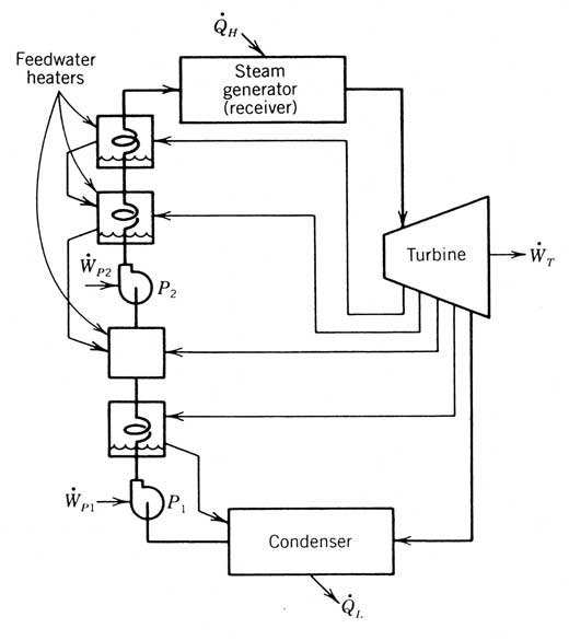
12.3
12.3.1
Cycle Description
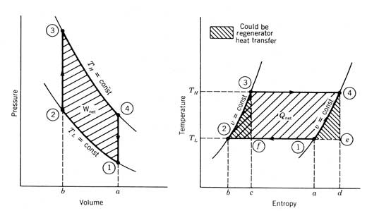
2
b
a
on the pressure-volume (p-v) diagram and the amount
of heat transferred from the working fluid, by area 1-2-b-a on the
temperature-entropy (T
s) diagram. The next process is the constant-volume heat
addition process (2
3),
where the temperature is raised from TL
to
TH and there is no work done. The heat addition is represented by the area
2
3
c
b
in the T
s
diagram. Following this is the
constant-temperature expansion process (3
4),
where work is done by the working fluid as heat is added. The work is represented by the area b-3-4
a
in the
p
ν diagram and the heat addition by area c
3
4
d
in the T-s
diagram. The cycle is closed by a
constant-volume heat rejection process (4
1),
where no work is done and the heat rejected is represented by area a
1
4
d
in the T-s diagram.
2
3
4
in the p
v
diagram in Figure 12.22. By the first
law of thermodynamics, this is also the net amount of heat that must be added
to the cycle to produce this work. This net amount of heat is represented by
the area 1
2
3
4
in the T-s
diagram.
3
and 4
1. Because these processes represent an equal
amount of heating and cooling of the working fluid with no work involved, a
regenerator may be used that saves the heat represented by area 1
4
e
in the
T-s diagram and transfers it to the working fluid during the
compression process 2
3
as represented by area 2
3
f
on the same diagram. By eliminating the
need to transfer heat from an external source at temperatures other than the
maximum and minimum cycle temperatures, the regenerative
heat
rejection
process (1
2),
the work done on the gas is
(12.17)
R
is the universal gas
constant,
the molecular weight of the gas, and m
is the mass. The value will be negative
because of the sign convention that work done on the cycle is negative. The amount of heat transfer for this process
is the same since there is no change of temperature of the gas:
(12.18)
(12.19)
(12.20)
(12.21)
(12.22)
(12.23)
12.3.2 Real
Engine Analysis

volume
plot of a real cycle and how the cycle might be implemented by use of an
alpha-type arrangement. There are three
important factors that make the actual cycle diagram resemble Figure 12.24 more
than Figure 12.22. These are sinusoidal
motion of the pistons, imperfect regeneration, and dead volume. The effects of these factors on the cycle
design are discussed in the paragraphs that follow.

(12.24)
(12.25)
(12.26)
(12.27)
(12.28)
12.3.3 Engine
Design Features
12.3.4 The
Solar 4-95 Engine

12.3.5 Free-Piston

12.4 Brayton
Cycle Engines
12.4.1 Ideal
Brayton Cycles
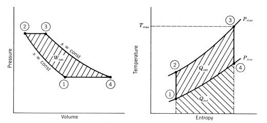
entropy
coordinates given in Figure 12.27 as the area under the process curves. The heat added to the cycle being the total
crosshatched area and the heat rejected, the area under process 4
1. The net amount of heat added to the cycle is
represented by the area enclosed by the processes. Similarly, the net work done by the cycle is
represented by the enclosed area on the pressure-volume coordinates.
(12.29)

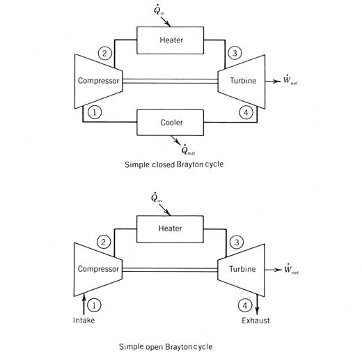
3
at atmospheric pressure and process 4-1 at sub-atmospheric pressure has been
proposed. The major advantage of this cycle concept is that the receiver does
not have to withstand high-pressure differences, providing for less structure
and thinner heat or optical transfer surfaces.
An example of this concept, the SABC, is discussed below.

(12.30)
(12.31)

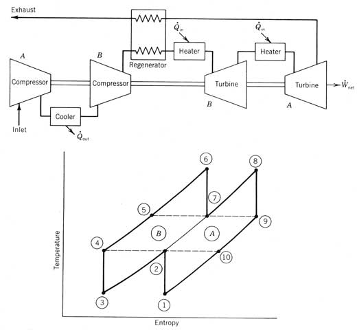
12.4.2 Real
Engine Processes
(12.32)
5
and 4
5s.

(12.33)
(12.34)
12.4.3 Cycle
Analysis
12.4.4 The
SABC Solar Engine


12.4.5 The
SAGT Solar Engine

12.5 Solar
Combined With Fossil Fuel Power Cycles
12.5.1
Solar Energy for Boosting Combined Cycles

Figure 12.36 Relative CO2 emissions of fossil and hybrid power plants.
Only the integration of solar fields into combined cycle systems will also maintain the fuel saving and emission reduction advantage of solar thermal plants over any kind of fossil cycle in the future. In such a configuration the solar field would boost the high fuel efficiency of these upcoming combined cycles with further significant enhancement.
Figure 12.37 illustrates the temperature differences between the exhaust-gas hot stream and the steam/water streams along the flow path of single, dual and triple pressure waste-heat recovery boilers. Since solar steam generators with single-phase air, molten salt and oil heat-transfer media have pinch-point problems similar to a waste-heat recovery boiler, their curves are also included in Figure 12.37.

Figure 12.37 Heat transfer in fossil-fueled, combined cycle power plants with waste heat recovery boilers.
The approach of the exhaust-gas or solar heat-transfer medium to the saturation temperature - the “pinch point” - strongly influences the magnitude of the area required for heat transfer in the unit. In all these sensible heat steam generators, 60-70% of heat transfer occurs in the steam generation section(s) at a boiling point under 400°C, while only 15-20% of the heat transfer occurs above 400°C in the superheaters and reheaters.
In a conventional combustion turbine combined cycle plant such as the one shown in Figure 12.38 the waste heat from the Brayton cycle is used to generate and superheat steam for the Rankine cycle in the waste heat recovery system. The steam turbine may operate at an efficiency as low as 24% due to steam pressure and temperature restrictions caused by the admissible moisture content in the final expansion stages.
Figure 12.38 Schematic flow diagram of a conventional fossil-fueled combined cycle power plant
In a conventional steam plant, much higher efficiencies are possible through high superheat and/or reheating, but in a pure combined cycle steam pressure is restricted to 40-60 bar at superheat temperatures of 480-500°C and reheating is not possible since insufficient energy is available at high temperatures. Exhaust gas temperatures exiting the waste heat recovery system may be undesirably high (increasing exhaust heat losses) depending on fuel type and the number of steam pressure levels (dual or triple levels are more complex, but increase efficiency). Confronted with this constraint, waste-heat recovery boilers are faced with trade-offs in the selection of the pinch point in a particular design or application. Typical steam outlet conditions for waste heat recovery heat exchangers (WHR-HX) for a conventional fossil-fueled combined cycle power plant are given in Figure 12.39.
Figure 12.39 Steam outlet conditions for waste heat recovery heat exchangers (WHR-HX) for a conventional fossil-fueled combined cycle power plant.
If a solar field is added in parallel with a waste-heat recovery boiler in a combined cycle system as illustrated in Figure 12.40, feeding only intermediate pressure steam into a corresponding steam turbine system inlet, nothing of the classical pinch point problem has been changed.
Figure 12.40 Parallel connection of a solar field and a waste heat recovery boiler.
A parabolic trough solar field with about 400°C outlet temperature could ideally take over the steam generation function, so that the design of the waste-heat recovery boiler is no longer dependent on the pinch point as a design constraint and a higher heat recovery factor can be achieved. With no pinch point, the flue gases can be cooled down to a lower temperature (116°C instead of 180-200°C) and more energy can be extracted from them.
Exhaust heat from the gas turbine is now used more effectively from the viewpoint of the 2nd law of thermodynamics, since it is largely input into the cycle at a higher temperature (superheat section). In such a combined cycle configuration, the high temperature advantage of central receiver systems is much less important, since the solar function of steam generation requires only temperatures of about 400°C, while the required high temperature superheat is provided much more economically by the “free” gas turbine exhaust.
Integration of a solar system into a combined cycle, as shown in Figure 12.41, improves the steam parameters and permits the use of a reheated steam turbine. Consequently, steam cycle efficiency increases towards 40%, the overall plant efficiency rises and emissions are reduced. In the integrated solar combined cycle plant, the gas turbine cycle is unchanged. However, steam conditions are met by using solar heat to generate and reheat the steam and combustion turbine exhaust heat to both preheat the feedwater and superheat the steam.

Figure 12.41 Function sharing between a solar field and a waste heat recovery boiler.
Since no superheating is required from the solar system, the evaporation temperature can be raised so that steam pressure is higher, e.g., 100 bar. The combustion turbine exhaust is then used to superheat high pressure steam to a temperature as high as 500°C. The steam turbine capacity of the combined cycle is increased considerably due to the additional energy from the solar system. For example, a conventional combined cycle with a gas turbine capacity of 60 MWe would utilize a steam turbine of about 30 MWe capacity, whereas in the ISCCS design steam turbine capacity is about 80 MWe. Temperature profiles for a) a conventional power plant with waste heat recovery and b) the waste heat recovery system in an integrated solar and combined cycle system are shown in Figure 12.42.
Figure 12.42 Temperature profiles for a) a conventional power plant with waste heat recovery and b) the waste heat recovery system in an integrated solar and combined cycle system.
Therefore, a combined-cycle solar parabolic-trough plant configuration is currently proposed by Pilkington Solar International for commercial power generation - the ISCCS (Integrated Solar
and Combined Cycle System) concept shown in Figure 12.43.

Figure 12.43 The proposed Pilkington integrated solar and combined cycle system
(ISCCS) incorporating a gas turbine plus 100% solar field. (courtesy Pilkington
Solar International,
SEGS steam cycle plants have been constructed in capacities ranging from 15 to 80 MWe net, and conceptual designs have been developed up to 200 MWe capacity. It is generally true that reasonable costs can be achieved at 30 MWe and above, though the larger sized plants clearly benefit from economies of scale, and thus are more economically attractive. Based on existing plant designs and current SEGS experience, an 80 MWe plant is considered to be the reference configuration. When a solar system is coupled with a combined cycle in the ISCCS configuration, overall plant capacities can reach over 200 MWe without extending beyond the current experience with SEGS-type solar fields. Selection of the plant size at each site depends, of course, on the capacity requirements and electrical grid structure in that area.
12.5.2 Minimizing CO2 Emissions
CO2 emissions from fossil-fired power plants are directly proportional to fuel consumption, and are thus inversely proportional to the efficiency of the fossil-fired conversion cycles. The combination of solar fields and gas-fired combined cycles results in the minimization of fuel use and, accordingly, the minimization of CO2-emissions. The solar field may be regarded as a subsystem enhancing fuel efficiency in the same way classical improvements of thermal cycles did, e.g., economizers, preheating, feedwater heaters, and reheat.
Figure 12.44 shows the kWh-specific CO2 emissions of various
conversion technologies for several fossil fuels contributing to the 1990
Mediterranean Area average emissions of 0.92 kg CO2 per kWh. Even with the 40% conversion efficiency of
modern steam cycles, coal plants still emit 0.9 kg CO2 per kWh. In order to further
decrease these emissions, new technologies with enhanced conversion
efficiencies, such as the integration of pressurized fluidized bed coal
combustors in the 305 MW IGCC project in
The specific investment costs of US $1,920 per kW installed for this first-of-a-kind demonstration project are being shared by electricity generating companies of five EU countries and the EU. However, the lowest CO2 emissions of 0.4 kg CO2 per kWh are emitted by 50%-efficient natural gas-fired combined cycles. Even greater improvement can be achieved by the integration of solar technology into this cycle.
Depending on the solar field size, solar irradiation and
operation strategy, average emissions from the mixed solar/fossil ISCCS
operation can yield 0.1 to 0.3 kg CO2
per kWh, while the pure solar operated SEGS has zero emissions. Parabolic
trough solar power plants have an average CO2 reduction capacity of approximately 150 to 200 kg CO2/year per m
of installed solar field, depending on solar irradiation and operating mode.

Figure 12.44 Comparison of specific CO2 emissions of various conversion
technologies. (Courtesy of Pilkington Solar International,
Depending on the size of the solar field and the resulting solar share of production, the equivalent solar-enhanced fuel efficiency, that is, annual net electric output divided by the lower heating value of the fuel consumed in this period, can be raised to over 80%. Thus the combination of proven gas-fired combined cycle technology with proven parabolic trough solar thermal technology offers a particularly attractive fossil thermal power plant technology for the next decade.
12.5.3 Electricity Yield and Costs
The SEGS projects in
By integrating proven solar field technology into the most fuel efficient and advanced combined cycle power conversion technology, hybrid solar/fossil-fired thermal power plants are able to supply base-load or mid-load power. Performance and, subsequently, electricity cost results depend on the plant contractor's operating demand scenario.
To illustrate this, a representative mid-load demand termed the regional demand, is presented here. It is typically comprised of full-load operation during the weekday daylight hours, part-load on weekday evenings and nights, and solar-only during weekends and holidays. This regional demand profile results in up to about 4,500 hours per year of full load operation. Performance runs for the Mediterranean region were carried out using an hour-by-hour solar plant model developed by FLAGSOL, and validated with operating data obtained from the SEGS plants operated by the Kramer Junction Company, comparing very well at a detailed level between projected and actual results.
The performance of the solar fields and ISCCS plants vary somewhat depending on size and site, but in general in the Mediterranean region annual solar field thermal efficiency is about 45%, an annual solar-to-electric efficiency based on normal direct solar irradiation of about 14-15%, and an annual solar energy production of about 800-900 kWh/m2 (thermal). This same solar field performance is found in the ISCCS plants, with the electrical output dependent on combined cycle performance as a function of load. Standard methods were used to calculate the LEC (Levelized Electricity Cost) - e.g. the LEC was based on the International Energy Agency method with the following economic boundary conditions: 6.1% discount rate, 1% insurance rate, 38% income tax, 6.7% depreciation, 3% interest rate on loans during construction, 4% fuel and general cost escalation rate and 3% electricity tariff escalation rate.
Levelized electricity costs for an 135 MWe ISCCS system in
southern Spain are estimated to be 8.3 US cents / kWh in the regional demand
case (3500 equivalent full-load hours) and 6.8 US cents / kWh in the base load
case (6000 equivalent full load hours). For comparison, a standard 80 MWe SEGS
station in
12.5.4 Conclusions
Pure solar thermal electricity generation of 2000 to 3000 full-load hours must not only bear the solar equipment investment, but also pay the extra cost of improving the conventional power block equipment. Even if the solar system were free of cost, any client electric utility would therefore seek to operate the costly power block beyond pure solar operation for as many hours as possible with additional fossil firing. Fossil-firing just to minimize the power-block-related generating costs, is between 2000 and 5000 annual full-load hours.
The integration of a solar field into a combustion/steam-turbine combined cycle increases the effectiveness of solar input in the integrated mode, enhances the thermodynamic efficiency of the combined cycle and reduces the emissions per MW output of the overall system compared to a conventional combined cycle. The solar energy itself is used in steam turbines with comparable efficiencies, but the fossil-fuel contribution is much more effective in the combined cycle and thus the annual performance is significantly enhanced in the mid and base-load operation. Depending on the size of the solar field, solar irradiation and operating strategy, average emissions from the mixed solar/fossil ISCCS can yield as little as 0.1 to 0.3 kg CO2 per kWh.
The solar field may be regarded as a subsystem which enhances fuel efficiency just as classical thermal cycle improvements, such as economizers, preheating, feedwater heaters, and reheat. The equivalent solar-enhanced fuel efficiency, that is, annual net electric output divided by the lower heating value of the fuel consumed in this period, can be raised to over 80%. Levelized electricity costs for the 135 MWe ISCCS system in southern Spain are 8.3 US cents / kWh in the regional demand case (3500 equivalent full load hours) and 6.8 US cents / kWh in the base load case (6000 equivalent full load hours).
References
Abbin, J. P. and W.R. Leuenberger (1974), “Program CYCLE: A Rankine Cycle Analysis Routine,” Sandia National Laboratories Report SAND 74-0099 (revised).
Abbin, J. P. (1983), private communication.
Baljé, O. E. (1962), “A Study On Design Criteria and
Matching of Turbomachines: Parts A and B," Transactions of the ASME;
Journal of Engineering Power, 83114,
January.
Bowyer, J. M. (1983), private communication.
Bowyer, J. M. (1984), “The Kinematic
Harrigan, R. W. (1978),"Solar Total Energy Systems Design", Sandia National Labs, Report SAND 78-0449, August,
Marciniak, T. J., J. L. Krazinski, J. C. Bratis, H. M. Busby, and E. H. Buyco (1981), “Comparison of Rankine-Cycle Power Systems: Effects of Seven Working fluids,” Argonne National Laboratory Report ANL/CNSV-TM-87, June.
Martini, W. R. (1980), “
Reynolds, W. C, (1979), “Thermodynamic Properties in Sl;
Graphs, Tables and Computational Equations for Over 40 Substances,” Department
of Mechanical Engineering,
Roschke, E.J., L. Wen, H. Steele, N. El Gabalawi, and J. Wang (1979), “A Preliminary Assessment of' Small Steam Rankine and Brayton Point-Focusing Solar Modules," Jet Propulsion Laboratory Publication 79-21 (DOE/JPL -1060-16), March 1.
Schmidt, G., P. Schmid, H. Zewen and
Stine, W. B. (1984),"Survey of Manufacturers of High Performance Heat Engines Adaptable to Solar Applications," Jet Propulsion Laboratory Report JPL 84-46 (DOE/JPL-1060-75), June 15.
Tabor, H. (1962), “Solar Utilization and Development in
Urieli,
Related Studies and References
Anonymous (1988) "Solar Electricity Generating Systems" Pilkington Solar International, Köln 1988.
Geyer, M., H. Klaiß (1989) "194 MW Solarstrom mit Rinnenkollektoren" BWK Nr. 6 , Seite 288/95.
Aringhoff, R. (1990) "Solarthermische Kraftwerke in Kalifornien", ET (Energiewirtschaftliche Tagesfragen, Nr. 4).
De Laquil, P., Kearney, D., Geyer, M., Diver, R. (1993) "Solar-Thermal Electric Technology", Chapter 5 in Renewable Energy - Sources for Fuels and Electricity, Island Press ISBN 1-781559-631396.
Klaiß, H., Staiß, F. (1993) Solarthermische Kraftwerke für den Mittelmeerraum, Springer-Verlag.
Anonymous (1993) World Energy Outlook International Energy
Agency (IEA), ISBN 92-64--13904-4,
Anonymous (1993) Energy for Tomorrow's World, World Energy
Council (WEC)
Anonymous (1994) "SEGS Technology Assessment and
Transferability to the